The Excel Window

Microsoft Excel is an electronic spreadsheet. You can use it to organize your data into rows and columns. You can also use it to perform mathematical calculations quickly, and to create charts. This tutorial teaches Microsoft Excel basics. Although knowledge of how to navigate in a Windows environment is helpful, this tutorial was created for the Excel novice.

This lesson will introduce you to the Excel window. You use the window to interact with Excel. To begin:

1. Start Microsoft Excel. The Microsoft Excel window appears.
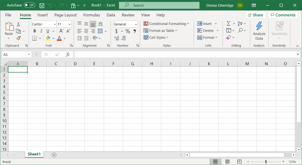
2. Click Blank Workbook. Excel opens a workbook. Your window should look like the one shown below.

Note: Your window will probably not look exactly like the screen shown. In Excel, how a window displays depends on the size of your window, the size of your monitor, and the resolution to which your monitor is set. Resolution determines how much information your computer monitor can display. If you use a low resolution, less information fits on your screen, but the size of your text and images are larger. If you use a high resolution, more information fits on your screen, but the size of the text and images are smaller. Also, settings in Excel and settings in Windows allow you to change the style of your windows.

There are several parts to the Excel window. I will explain them, starting from the top.

A AutoSave: When AutoSave is on, Excel saves your file to OneDrive every few seconds. When you save your file to OneDrive, it is accessible from any device. Also, AutoSave enables collaboration features which allow others to see who is working on a workbook and the changes they are making in real time.

B The Quick Access Toolbar: The Quick Access toolbar gives you access to commands you frequently use. By default, Save, Undo, and Redo appear on the toolbar. You can use Save to save your file, Undo to roll back an action you have taken, and Redo to reapply an action you have rolled back. You can add additional items to the Quick Access toolbar.

C The Title Bar: Microsoft Excel displays the name of the workbook you are currently using on the Title bar. At the top of the Excel window, you should see "Book1 - Excel" or a similar name. When you save your workbook, you will rename it.

D Search: You can use the Search box to find commands, issue commands, search for text, or find help on a command you do not understand.

E Account Access: You can use account access to sign into your account. Once you have accessed your account, you can view and edit your personal information, view a list of your subscriptions, change your password, and more.

F Ribbon Display Options Button: You can use the Ribbon Display Options Button to display the following menu options: Auto-hide Ribbon, Show Tabs, and Show Tabs and Commands. To learn more about these options, see the section The Excel Ribbon.

G Minimize Button: To remove Excel from view and place the Excel icon on the Windows taskbar, click the Minimize button. To restore Excel, click the Excel icon on the Windows taskbar.

H Restore Down: The Restore Down button reduces the size of the Excel window. When you click the Restore Down button, it turns into the Maximize button.

Maximize Button: The Maximize button fills your screen with the Excel window. When you click the Maximize button, it turns into the Restore Down button.

I Close Button: The Close button closes the active workbook. When you click the Close button, if you have not previously saved your workbook or if you have made changes to your workbook since you last saved, a dialog box opens. Click Save if you want to save your changes, Don’t Save if you do not want to save your changes, or Cancel if you have decided not to close your workbook. If the workbook you are closing is the only workbook open, the Close button also closes Excel.

The Ribbon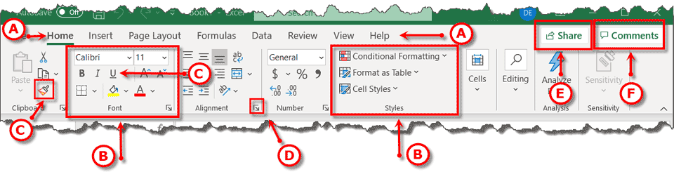

You use commands to tell Microsoft Excel what to do. You use the Ribbon to issue commands. The Ribbon is located near the top of the Excel window, below the Quick Access toolbar.

A Tabs: At the top of the Ribbon are several tabs; clicking a tab displays several related command groups.

B Command Groups: A command group is a group of related command buttons. Each tab has several command groups.

C Command Buttons: Within each group are related command buttons. You click buttons to issue commands or to access menus and dialog boxes.

D Dialog Box Launcher: You may find a dialog box launcher in the bottom-right corner of a group. Click the dialog box launcher to see additional commands in a dialog box or pane.

E Share: Clicking the Share button opens a dialog box that allows you to login to OneDrive and save your file there. You can also give others permission to access and/or edit your document.

F Comments: Click the comments button to add or review comments.

The Ribbon Display Options Button

The Ribbon Display Options Button  is located in the upper right corner of the window. When you click it, the following options appear:

Auto-hide Ribbon:

Choosing this option completely hides the Ribbon. Once the Ribbon is hidden, clicking  displays the Ribbon. With the Ribbon displayed, you can select cells. Click , and then select a Ribbon option. Excel will apply the option. You can then click anywhere on the worksheet to hide the Ribbon again.

Show Tabs:

Choosing this option shows the Tabs but not the Command Groups. You can select cells, click a Tab, and then select a Ribbon option. Excel will apply the option. You can then click anywhere on the worksheet to hide the Ribbon again.

Show Tabs and Commands:

This is the default option. When this option is selected, both the Tabs and the Command Groups always display.

Unpinning and Pinning the Ribbon

As you work, the Ribbon can be either pinned or unpinned. When the Ribbon is pinned, tabs and command groups are visible. When the Ribbon is unpinned, you can see the tabs but not the command groups—when you click a tab, the command groups appear.

Unpin the Ribbon

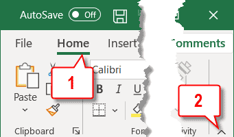
1. Choose any tab. The Ribbon appears.
2. Click the chevron in the lower-right corner of the Ribbon. Excel unpins the Ribbon. You can now see the tabs but not the command groups. This is the same as clicking the Ribbon Display Options Button and then selecting Show Tabs.

Note: The chevron only appears when the Ribbon is pinned.

Pin the Ribbon

1. Choose any tab. The Ribbon appears.
2. Click the pin in the lower-right corner of the Ribbon. Excel pins the Ribbon. You can see both the tabs and the command groups. This is the same as clicking the Ribbon Display Options Button and then selecting Show Tabs and Commands.

Note: The pin only appears when the Ribbon is unpinned.

Are there other ways to pin and unpin the Ribbon?

Yes. Right-click on the Ribbon, then on the menu that appears, click Collapse the Ribbon. If the Ribbon is pinned, clicking this option will unpin it. If the Ribbon is unpinned, clicking this option will pin it.

How can I find out what each button on the Ribbon does?

When you hover over a button, Excel displays the name of the button, a description of the button’s function, and if a shortcut key is associated with the function, Excel displays the shortcut key.

If you do not see a button name and/or a description, the setting that causes the button name and/or description to display is turned off. To turn these features on:

1. Choose the File tab. A menu appears along the left side of the window.
2. Click Options. The Excel Options dialog box opens. A menu appears along the left side of the dialog box.
3. Choose General.
4. Under User Interface Options, click the down-arrow next to the ScreenTip Style field. Excel presents the following options: Show Feature Descriptions in ScreenTips, Don’t Show Feature Descriptions in ScreenTips, and Don’t Show ScreenTips. Click the option you want—for a description of each option, see the following ScreenTip Styles table.
5. Click OK to make your changes and close the dialog box.

ScreenTip Styles
Option	Description
Show Feature Descriptions in ScreenTips	Displays the button name and a description of the button’s function
Don’t Show Feature Descriptions in ScreenTips	Displays the button name but does not display a description of the button’s function
Don’t Show Screen Tips	Does not show Button Names or Screen Tips

The Formula Bar and Worksheets

Optionally, the Formula Bar is found below the Ribbon.

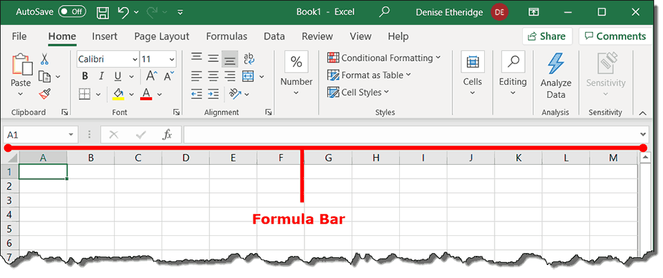
You can use the Formula Bar to enter and edit data. The current cell address displays in the Name box to the left of the Formula bar. If your Formula Bar is not visible, follow the steps listed here:

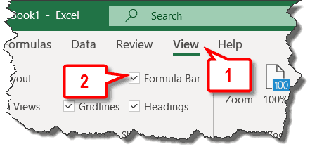
1. Choose the View tab.
2. Click to check the Formula Bar box in the Show group. Excel displays the Formula Bar.

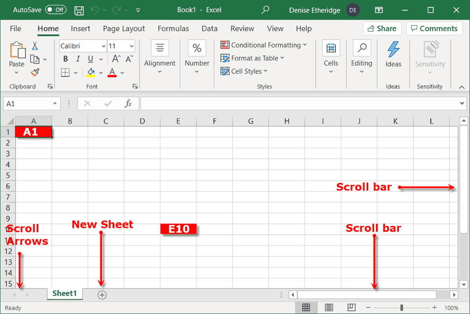
Microsoft Excel consists of worksheets. Each worksheet contains columns and rows. The columns are lettered starting with A to Z and then continuing with AA, AB, AC and so on. The rows are numbered starting with one, and continuing two, three, four. Only your computer memory and your system resources limit the number of columns and rows you can have in a worksheet.

Worksheets are divided into cells. The combination of a column coordinate and a row coordinate make up a cell address. You refer to cells by their cell address. For example, the cell located in the upper left corner of a worksheet is called cell A1, meaning column A, row 1. Column E10 is located under column E on row 10. You enter your data into the cells in the worksheet.

Scroll bars are located to the right of and below the worksheets. You can move up, down, and across your window by dragging the icon located on a scroll bar. The vertical scroll bar is located along the right side of the window. The horizontal scroll bar is located just above the Status bar. To move up and down your worksheet, click and drag the icon on the vertical scroll bar, up and down. To move back and forth across your workbook, click and drag the icon on the horizontal scroll bar, back and forth.

Each Excel file is a workbook. Each workbook can have multiple worksheets. To add a worksheet, click the New Sheet icon. You can use the Scroll Arrows to scroll through your worksheets.

The Status Bar

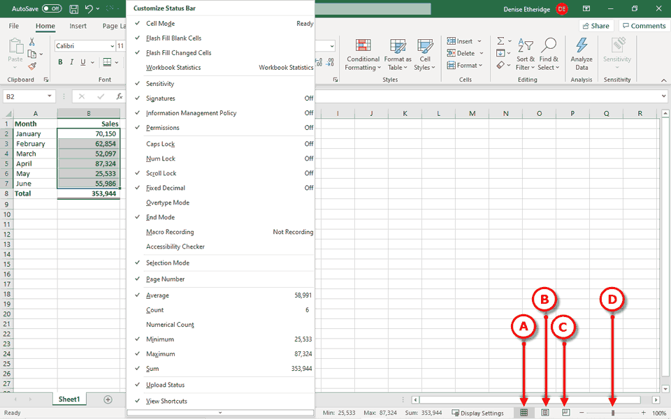
The Status bar appears at the very bottom of the Excel window and provides such information as the sum, average, minimum, and maximum value of selected numbers. You can change what displays on the Status bar by right-clicking on the Status bar and selecting the options you want from the Customize Status Bar menu. You click a menu item to select it. You click it again to deselect it. A check mark next to an item means the item is selected.

A Normal Button : The Normal button formats your worksheet for easy data entry.

B Page Layout Button : The Page Layout button displays your workbook in such a way as to make it easy for you to assign printing options and to see how your worksheet will look when printed.

C Page Break Preview : The Page Break Preview button displays your workbook and shows where each page begins and ends.

D Zoom Slider and Zoom: The Zoom slider zooms in and out on your workbook. Dragging the slider to the left zooms out, makes your workbook smaller, and allows you to see more of your workbook. Dragging the slider to the right zooms in, makes your workbook larger, and reduces the amount of your workbook you can see. The Zoom slider appears on the Status bar if Zoom Slider is selected on the Status bar menu. The percentage of zoom appears to the right of the zoom slider, if Zoom is selected on the Status bar menu.